Why CVXPY
What is CVXPY
CVXPY is Python-based domain-specific language (DSL) for convex optimization problems. To use a convex optimization problem in an application, it is needed to develop a costum solver or convert the problem into a standard form required by the solvers. An alternative is to use a DSL like CVXPY that lets the modeller to express an optimization problem in a natural way that follows the math. CVXPY helped us to add a lot if potentials to the Hypatia framework. One of the most salient ones is the possibility to include two dimensional variables and parameters in the model which allow us to construct element-wise vector and matrix-based equations. To be more specific, rather than using scalar-based mathematical equations that are mostly used in Pyomo-based energy optimization models, Hypatia uses element-wise matrix-based equations which help to bypass most of the rquired for loops on some of the structural inputs (sets) of the energy model such as the modelling years, technologies and more importantly the timesteps defined within each year of the time horizon. Therefore it is possible to say that “vectorized” problems are less time consuming compared to “scalar-based” problems in terms of building and passing the model to the solver.
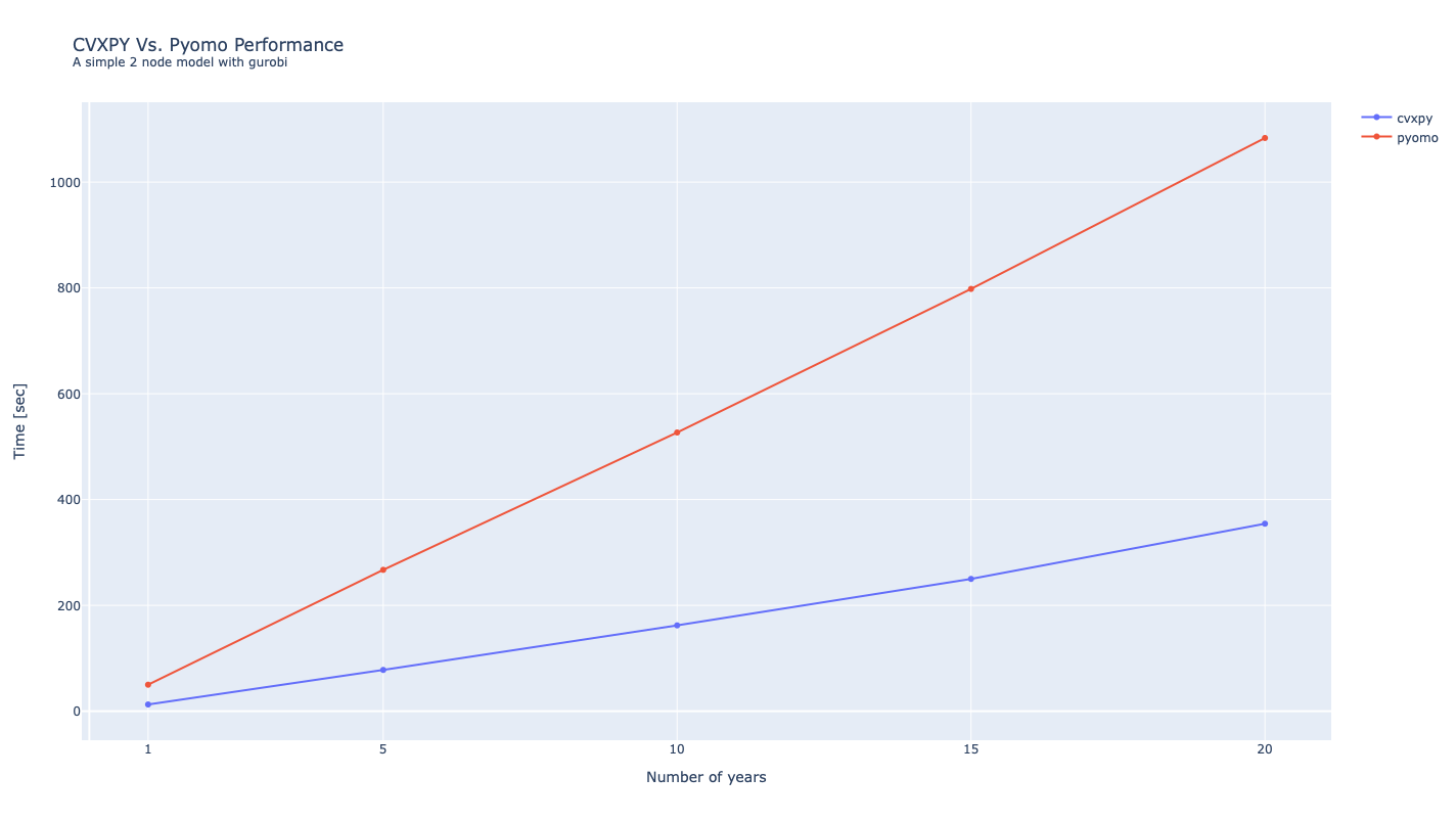
In this document, we compare the performance of CVXPY vs. Pyomo that is the most popular Python optimization library for the energy modellers. To test the performance of these two optimization libraries in terms of the required time to build a unique model, A dummy two-node energy system application with hourly time resolution and annual capacity expansion is created in both Pyomo and CVXPY langiages. We configure the solvers to terminate immidiately after one single iteration to avoid considering the time required to solve the problem and, therefore, only the time required to generate and load the problem to the solver has been investigated. Moreover, through this example, one can also understand how defining an optimization problem in CVXPY is more convinient and transparent than in Pyomo. Tnis feature of CVXPY helps energy modellers without professional coding skills understand the models and contribute to the development easier.
Note
The data of the test along with its jupyter notebook script are available in GitHub.
Pyomo Version
model = AbstractModel()

# Definition of sets
model.years = Set(initialize=lambda model: years)
model.hours = Set(initialize=lambda model: hours)
model.techs = Set(initialize=lambda model: techs)
model.regs = Set(initialize=lambda model: regions)

# Definition of Vars
model.production = Var(
    model.years, model.hours, model.techs, model.regs, domain=NonNegativeReals
)
model.new_capacity = Var(
    model.years, model.techs, model.regs, domain=NonNegativeReals
)
model.total_capacity = Var(
    model.years, model.techs, model.regs, domain=NonNegativeReals
)
# Definition of paramters
model.inv_cost = Param(
    model.years,
    model.techs,
    model.regs,
    initialize=lambda model, y, t, r: inv_cost.loc[y, t],
)
model.var_cost = Param(
    model.years,
    model.techs,
    model.regs,
    initialize=lambda model, y, t, r: var_cost.loc[y, t],
)

model.availability = Param(
    model.years,
    model.hours,
    model.techs,
    model.regs,
    initialize=lambda model, y, h, t, r: availability.loc[(y, h), t],
)
model.demand = Param(
    model.years,
    model.hours,
    model.regs,
    initialize=lambda model, y, h, r: demand.loc[(y, h), "demand"],
)

# Definition of rules
def tot_cap(model, y, t, r):
    if y == years[0]:
        return model.total_capacity[y, t, r] == model.new_capacity[y, t, r]
    return (
        model.total_capacity[y, t, r]
        == model.total_capacity[y - 1, t, r] + model.new_capacity[y, t, r]
    )

def demand_prod(model, y, h, r):
    return (
        sum(model.production[y, h, t, r] for t in model.techs)
        == model.demand[y, h, r]
    )

def availability_prod(model, y, h, t, r):
    return (
        model.production[y, h, t, r]
        <= model.total_capacity[y, t, r] * model.availability[y, h, t, r]
    )

def objective_function(model):

    tot_inv = sum(
        model.inv_cost[y, t, r] * model.new_capacity[y, t, r]
        for y in model.years
        for t in model.techs
        for r in model.regs
    )
    tot_var = sum(
        model.var_cost[y, t, r]
        * sum(model.production[y, h, t, r] for h in model.hours)
        for y in model.years
        for t in model.techs
        for r in model.regs
    )
    return tot_inv + tot_var

model.balance_rule = Constraint(
    model.years, model.hours, model.regs, rule=demand_prod
)
model.availability_rule = Constraint(
    model.years, model.hours, model.techs, model.regs, rule=availability_prod
)
model.capacity_rule = Constraint(model.years, model.techs, model.regs, rule=tot_cap)
model.OBJ = Objective(rule=objective_function, sense=minimize)

instance = model.create_instance()

opt = SolverFactory(solver)
CVXPY Version
constraints = []
tot_var_cost = 0
tot_inv_cost = 0

for rr in regions:
    # Creting variables
    production = cp.Variable(
        shape=(len(years) * len(hours), len(techs)),
        nonneg=True,
    )

    new_capacity = cp.Variable(shape=(len(years), len(techs)), nonneg=True)

    # meeting the demand
    constraints.append(
        cp.sum(production, axis=1) == demand.loc[years, "demand"].values
    )

    # total capacity -> cummulative sum of new capacity assuming
    # there is no disposed capacity
    if len(years) == 1:
        total_capacity = new_capacity
    else:
        total_capacity = cp.cumsum(new_capacity)

    # Production lower than the available capacity

    for yy, year in enumerate(years):
        constraints.append(
            production[yy * 8760 : (yy + 1) * 8760, :]
            <= cp.multiply(
                total_capacity[yy : yy + 1, :],
                availability.loc[(year, slice(None)), :].values,
            )
        )

        tot_var_cost += cp.sum(
            cp.multiply(
                cp.sum(production[yy * 8760 : (yy + 1) * 8760, :], axis=0),
                var_cost.loc[year, :].values,
            )
        )
    tot_inv_cost += cp.sum(cp.multiply(new_capacity, inv_cost.loc[years, :].values))

# Definition of objective function
objective = cp.Minimize(tot_var_cost + tot_inv_cost)

# Problem definition
problem = cp.Problem(objective=objective, constraints=constraints)
probblem.solve()
Results
As it is illustrated below, CVXPY always show a better performance in terms of time needed to pass the model to the solver. While for short time horizons, the difference is quite negligible, for long time horizon, the difference is so considerable.